Flux Limiters

Consider a conservation law such as $u_t = -au_x$, and the following schematic. We can also write this as $u_t = -f_x,$ where $f=au$ is the flux.

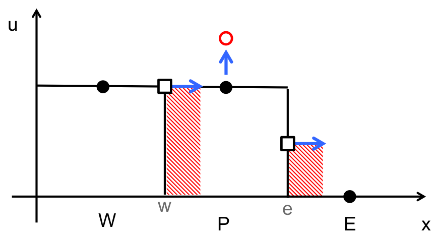
We have three cells: W, P, and E.
The initial profile is the black line where we have a square wave.
The cell center values of u(x) are noted by the filled black circles.
The east and west face center values are shown as open squares.
- From averaging the neighbors.

Now, consider what happens when the wave moves.

The exact solution is just translation.
The initial profile indicates that there should be no net accumulation in the P cell.
However, because the fluxes are evaluated at the e and w faces, and those faces are given by the location of the squares, we have But $f_w > f_e$, so we have more flux in than out, which is indicated by the red shaded regions. The result is an increase in the value of $u_P$. This is a problem, and it results in oscillations for the “standard” high order schemes.
Question: what about upwind?
Visualize the above schematic for upwind. What happens to cell P? Cell E? Consider in terms of the stepsize implied in the figure, and other step sizes.

Godunov’s Theorem

“Linear numerical schemes for solving partial differential equations (PDE’s), having the property of not generating new extrema (monotone scheme), can be at most first-order accurate.” (From Wikipedia)

This means that if you want to avoid wiggles, you have to use a first order method (like upwind),
- Unless you form a nonlinear scheme.
This is what flux limiters are designed to do.

Flux limiter description

Flux limiters limit the flux to avoid this oscillation. For $u_t = f_x$, (and a simple time integration) we have

$$ u_i^{n+1} = u_i^n - \frac{\Delta t}{\Delta x}(f_e^n-f_w^n).$$

We evaluate the flux at, e.g., the east face, as

$$f_e = f_e^{l} - \phi_e(r)(f_e^{l}-f_e^{h}) = (1-\phi_e(r))f_e^l + \phi(r)f_e^h.$$

This is a combination of two fluxes. $f_e^l$ is a low-order flux, such as an upwind flux (first order), and $f_e^h$ is a high order flux, such as a central or average flux (second order).

If we use upwind for $f_e^l$ and a central (average) flux for $f_e^h$, we get

$$f_e = \underbrace{f\_e^{(1)}}\_{\mbox{upwind}} - \phi\_e(r)\left(\underbrace{f\_e^{(1)}}\_{\mbox{upwind}} - \underbrace{\frac{f\_e^{(1)}+f\_e^{(2)}}{2}}\_{\mbox{average}}\right),$$

or,

$$f_e = f_e^{(1)} + \frac{1}{2}\phi_e(r_i)\left(f_e^{(2)} - f_e^{(1)}\right).$$

Here, $f_e^{(1)}$ is the upwind flux and $f_e^{(2)}$ is the downwind flux.
$\phi(r)$ is a flux limiter function, which interpolates (nonlinearly) between the low and high fluxes.
The quantity $r$ is given by

$$r_i = \frac{u\_{i}-u\_{i-1}}{u\_{i+1}-u\_{i}}.$$

$r$ is the ratio of successive slopes and is a measure of how smooth the solution is.
If $r=1$, we have a very smooth solution and we would want $\phi=1$, so that we get the high order flux.
If $r=0$, there is a large change in the profile and we want $\phi=0$ so that we use the low order flux, so that we do not get oscillations.

Define $\phi(r)$

The following graph shows regions where the function $\phi(r)$ can “live” so that the method will be “total variation diminishing” (TVD), and also be $O(\Delta x^2).$

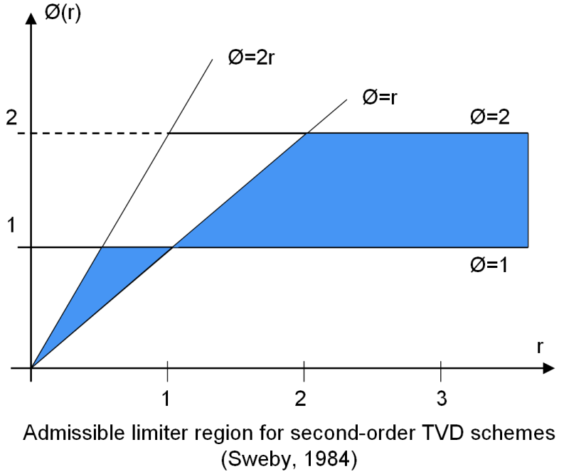
(From Wikipedia on 3/31/15, with the following license. No changes were made.)

There are many possible $\phi(r)$. Here is an example of a number of limiters (From Wikipedia on 3/31/15, with the following license. No changes were made.)

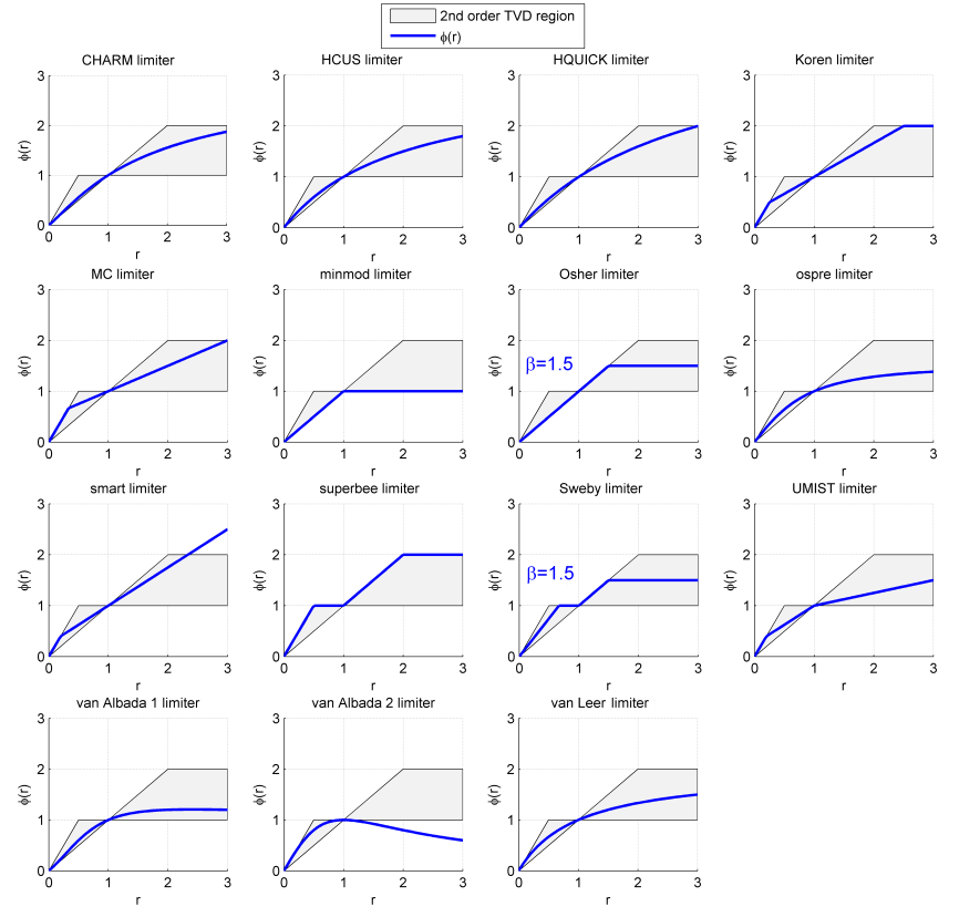
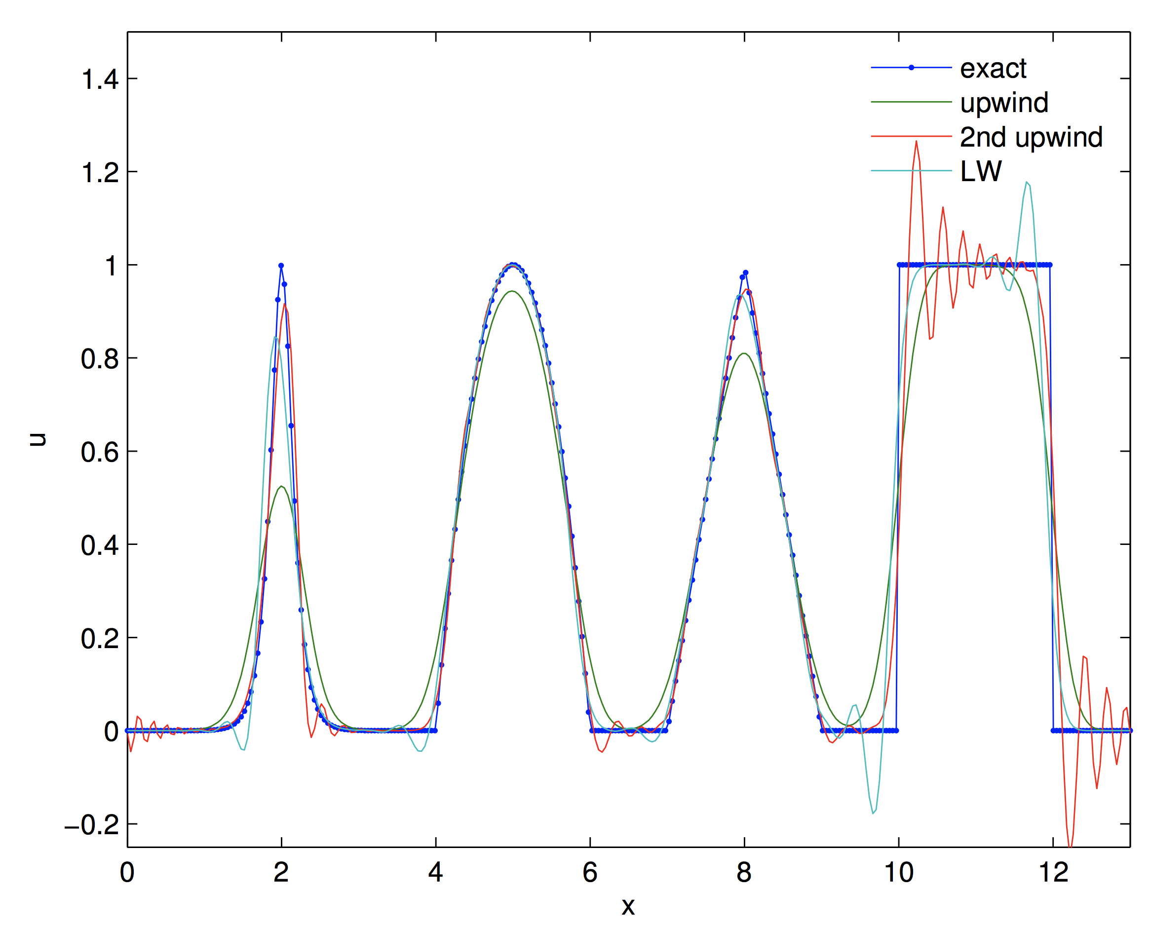
Consider 4 limiter functions

Superbee: $\phi(r) = \max(0,\min(2r,1),\min(r,2))$
Van Leer: $\phi(r) = (r+|r|) / (1+r)$
Minmod: $\phi(r) = \max(0,\min(r,1))$
MUSCL (MC): $\phi(r) = \max(0,\min(2r,1/2 + r/2, 2))$

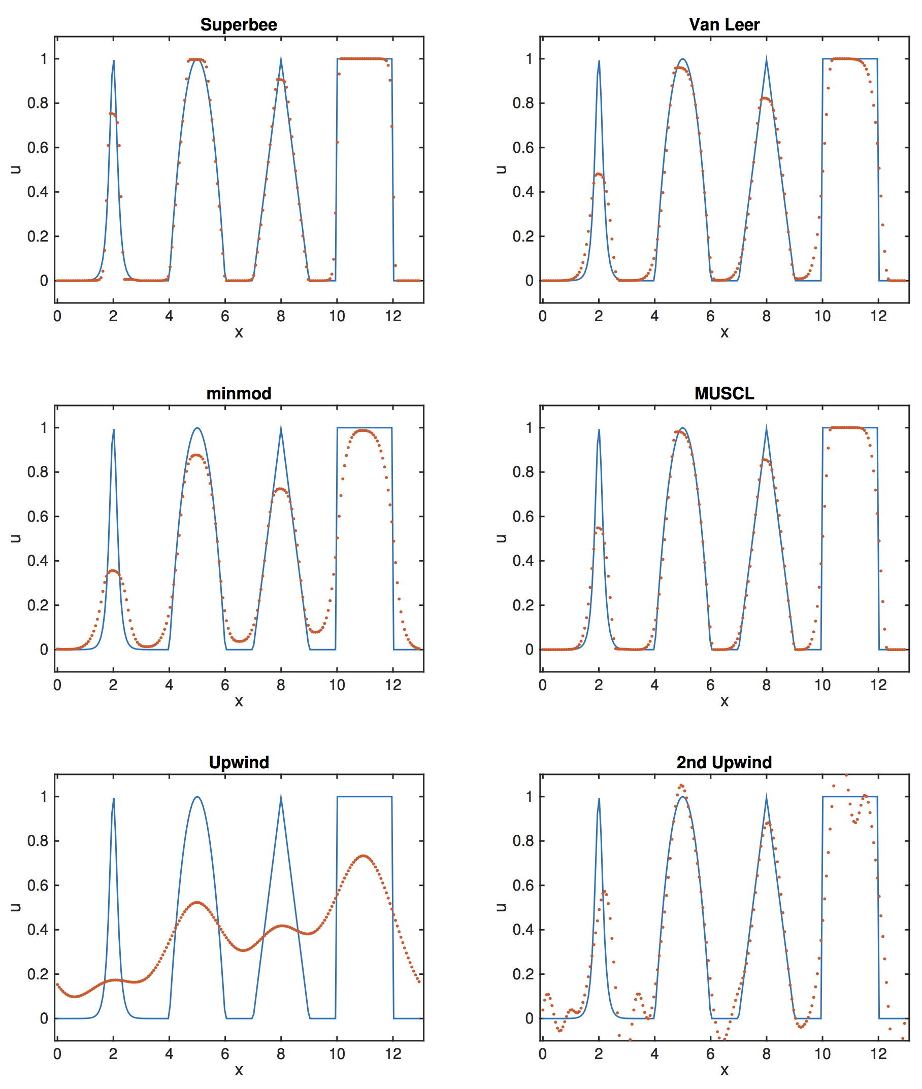
Note, the top four schemes are “high order.”
The lower two plots include schemes we have seen before.
The highly diffuse nature of the upwind scheme, and the oscillatory nature of the 2nd order upwind scheme, (which is high order, but not TVD).
The first four plots are TVD schemes and do not show oscillations.
Each method has a little different character.
Superbee does well, but tends to make peaks become square.

The above figure uses a 3rd order RK method, with 200 grid points and $cfl = a\Delta t/\Delta x = 0.4.$