Finite Volume Method

So far we have discussed PDEs and ODEs using the finite difference (FD) method.
- Set a grid of discrete points.

        *     *     *     *     *

Approximate the derivatives in the ODE/PDE at those points.
Solve for function values there.
Note, in FD, the starting point is the PDE.

Finite Volume (FV) method

Instead of a grid of points, make a grid of volumes.

      -------------------------------
      |     |     |     |     |     |
      -------------------------------

Insted of using the PDE (differential conservation law), use the integral conservation law.
- This is a standard balance on control volumes:
  - (accumulation) = (input) - (output) + (generation)

3 equivalent approaches.

Apply the above condition directly.
Integrate the PDE over a given control volume (CV).
Start from scratch and derive the governing equation from the conservation law (using the Reynolds Transport Theorem.)

Approach 1.

2-D unsteady heat transfer.
Energy balance
2-D grid
Control volumes i, j
Control faces: e, w, t, b.

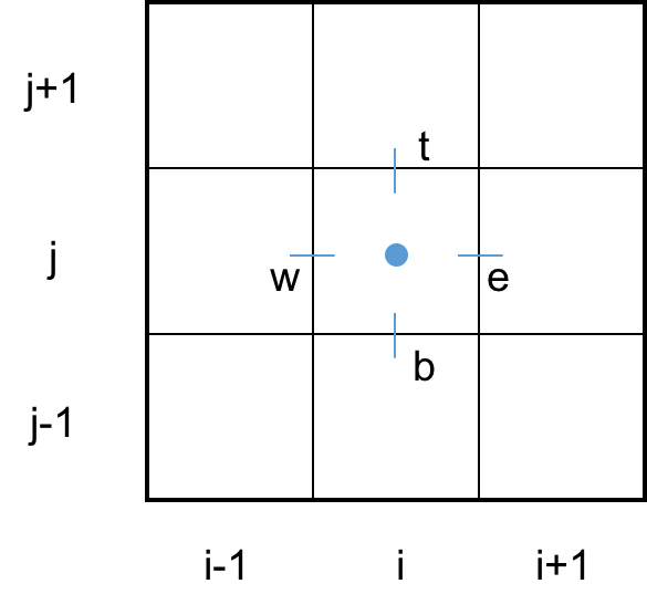
Assume properties are uniform throughout a given cell.
Assume properties are uniform along a cell face.
(accumulation) = (in) - (out) + (generation).

$$\frac{dE}{dt} = q_w\Delta y + q_b\Delta x - q_t\Delta x - q_e\Delta y + S\Delta x\Delta y.$$

* $E$ (=) J * $q$ (=) J/m$^2$s * $S$ (=) J/m$^3$s * $dE/dt = \Delta x\Delta y \rho c_pdT/dt.$

$$\color{blue}{\frac{dT_{i,j}}{dt} = -\frac{1}{\rho c_p}\left(\frac{q_{e,i,j}-q_{w,i,j}}{\Delta x_i}\right) - \frac{1}{\rho c_p}\left(\frac{q_{t,i,j}-q_{b,i,j}}{\Delta y_j}\right) + S_{i,j}.}$$

This equation is usually solved in this form, that is, in terms of fluxes.
Note, $q_{e,i,j} = q_{w,i+1,j}$.
Hence, energy is strictly conservered.
- This is an important property that is built-in to FV methods, but not necessarily for FD methods.
  - This is especially true for nonuinform grids with variable properties.

Evaluate the fluxes.

$$\vec{q} = q_x\vec{i} + q_y\vec{j},$$

$$q_x = -k\frac{\partial T}{\partial x},$$

$$q_e = -k\left.\frac{\partial T}{\partial x}\right|_e = -k\left(\frac{T_{i+1,j}-T_{i,j}}{\Delta x}\right),$$

$$q_w = -k\left.\frac{\partial T}{\partial x}\right|_w = -k\left(\frac{T_{i,j}-T_{i-1,j}}{\Delta x}\right),$$

$$q_t = -k\left.\frac{\partial T}{\partial y}\right|_t = -k\left(\frac{T_{i,j+1}-T_{i,j}}{\Delta y}\right),$$

$$q_b = -k\left.\frac{\partial T}{\partial y}\right|_b = -k\left(\frac{T_{i,j}-T_{i,j-1}}{\Delta y}\right).$$

If we substitute this into the governing equation, then on a uniform grid we obtain:

$$\frac{dT}{dt} = \frac{\alpha}{\Delta x^2}(T_{i-1,j}-2T_{i,j}+T_{i+1,j}) + \frac{\alpha}{\Delta y^2}(T_{i,j-1}-2T_{i,j}+T_{i,j+1}) + S_{i,j}.$$

This is the same equation as the FD method (for a uniform grid).
- The the approach is different.
- Nonuniform grids are common.
- Again, we normally solve the equation in terms of fluxes, not with the fluxes substituted into the governing equation.

Approach 2

Integrate the PDE over cell i, j

$$\frac{\partial T}{\partial t} = \alpha\frac{\partial^2T}{\partial x^2} + \alpha\frac{\partial^2T}{\partial y^2} + S,$$$$ \iint\frac{\partial T}{\partial t}dxdy = \iint\alpha\frac{\partial^2T}{\partial x^2}dxdy + \iint\alpha\frac{\partial^2T}{\partial y^2}dxdy + \iint Sdxdy, $$

$\partial/\partial t$ commutes with $\iint$.
Assume $T$, $S$, $\alpha$ are uniform:

$$\iint\frac{\partial T}{\partial t}dxdy = \frac{\partial}{\partial t}\iint Tdxdy = \frac{\partial}{\partial t}\left(T\iint dxdy\right) = \frac{\partial T\Delta x\Delta y}{dt} = \Delta x\Delta y\frac{\partial T}{\partial t}.$$

* Apply similarly for other terms.

Our equation now becomes

$$\Delta x\Delta y\frac{\partial T}{\partial t} = \alpha\Delta y\int\underbrace{\frac{\partial^2T}{\partial x^2}dx}_{ \int_{x_j}^{x_j+\Delta x_j}\frac{d}{dx}\left(\frac{\partial T}{\partial x}\right)dx \\= \left(\frac{\partial T}{\partial x}\right)_e-\left(\frac{\partial T}{\partial x}\right)_w}+ \alpha\Delta x\int\underbrace{\frac{\partial^2T}{\partial y^2}dy}_{ \int_{y_j}^{y_j+\Delta y_j}\frac{d}{dy}\left(\frac{\partial T}{\partial y}\right)dy \\= \left(\frac{\partial T}{\partial y}\right)_t-\left(\frac{\partial T}{\partial y}\right)_b}+ S\Delta x\Delta y.$$$$\Delta x\Delta y\frac{\partial T}{\partial t} = \Delta y\alpha\left(\frac{\partial T}{\partial x}\right)_e - \Delta y\alpha\left(\frac{\partial T}{\partial x}\right)_w + \Delta x\alpha\left(\frac{\partial T}{\partial y}\right)_t - \Delta x\alpha\left(\frac{\partial T}{\partial y}\right)_t + S\Delta x\Delta y.$$

(Again, repeating the previous equation)

$$\Delta x\Delta y\frac{\partial T}{\partial t} = \Delta y\alpha\left(\frac{\partial T}{\partial x}\right)_e - \Delta y\alpha\left(\frac{\partial T}{\partial x}\right)_w + \Delta x\alpha\left(\frac{\partial T}{\partial y}\right)_t - \Delta x\alpha\left(\frac{\partial T}{\partial y}\right)_t + S\Delta x\Delta y.$$

Now, using the following, etc., we obtain the same equation as approach 1.

$$\alpha\left(\frac{\partial T}{\partial x}\right)_e = -\frac{1}{\rho c_p}q_e,$$$$\color{blue}{\frac{dT_{i,j}}{dt} = -\frac{1}{\rho c_p}\left(\frac{q_{e,i,j}-q_{w,i,j}}{\Delta x_i}\right) - \frac{1}{\rho c_p}\left(\frac{q_{t,i,j}-q_{b,i,j}}{\Delta y_j}\right) + S_{i,j}.}$$

Approach 3

Use the Reynolds Transport Theorem (RTT).
The RTT is in the form: (generation) = (accumulation) + \[(out) - (in)\].
RTT:

$$\frac{dB}{dt} = \frac{d}{dt}\int_{CV}\rho\beta d\mathcal{V} + \int_{CS}\rho\beta\vec{v}\cdot\vec{n}d\mathcal{A}.$$

Here, $B$ is some extensive property (like total energy), and $\beta=B/m$ is the intensive property (like energy per unit mass).
Let $B=E$ and $\beta = E/m=e$.

$$\underbrace{\frac{dE}{dt}}_{(1)} = \underbrace{\frac{d}{dt}\int_{CV}\rho e d\mathcal{V}}_{(2)} + \underbrace{\int_{CS}\rho e\vec{v}\cdot\vec{n}d\mathcal{A}}_{(3)}.$$

In term (3), $\vec{v}=0$, no velocity, so term (3) = 0.
In term (2),

$$\frac{d}{dt}\int_{CV}\rho ed\mathcal{V} = \frac{d(\rho e\Delta x\Delta y)}{dt} = \Delta x\Delta y \rho c_p\frac{dT}{dt}.$$

In term (1) we apply the conservation law, which is the first law of thermodynamics:
$$\frac{dE}{dt} = \dot{Q} + \dot{W} + S\Delta x\Delta y.$$
- There is no work: no velocity, and constant $\rho$.
- For $\dot{Q}$, we have $$\dot{Q} = -\int_{CS}\vec{q}\cdot\vec{n}d\mathcal{A} = -\left[\int_b() + \int_t() + \int_e() + \int_w()\right] = -[q_e\Delta y - q_w\Delta y + q_t\Delta x - q_b\Delta x].$$
Now, substitute the terms back in (and flipping the equation order):
$$\Delta x\Delta y \rho c_p\frac{dT}{dt} = -[q_e\Delta y - q_w\Delta y + q_t\Delta x - q_b\Delta x] + S\Delta x\Delta y.$$
Rearranging, this gives the same equation as in the other methods:

$$\color{blue}{\frac{dT_{i,j}}{dt} = -\frac{1}{\rho c_p}\left(\frac{q_{e,i,j}-q_{w,i,j}}{\Delta x_i}\right) - \frac{1}{\rho c_p}\left(\frac{q_{t,i,j}-q_{b,i,j}}{\Delta y_j}\right) + S_{i,j}.}$$

Discussion

Note, we still use grid points when evaluating fluxes and properties. $$q_e = -k\frac{T_{i+1,j}-T_{i,j}}{\Delta x}.$$

Nonuniform grids

Two approaches, called practice A and practice B. (See Patankar’s book Numerical Heat Transfer and Fluid Flow).

Practice A

Faces are set midway between grid points:

    -----------------------------------------------------
    |   |                |              |        |      |
    *   |   *            |            * | *      |      *
    |   |                |              |        |      |
    -----------------------------------------------------

Better accuracy for fluxes (derivatives have symmetric central differences).
Has half a control volume at the boundaries
In 2-D, face values are not at the center of faces.

Practice B

Grid points are midway between cell faces:

    -------------------------------------------------------
    |   |   |             |                |        |      |
    | * | * |      *      |        *       |    *   |   *  |
    |   |   |             |                |        |      |
    -------------------------------------------------------

Center value is a better representation of the value in the CV. This is better for evaluating source terms.
Has a whole control volume at the boundaries